6.4-6.7 Intervals, Cantor set, density, and well-ordering

Chapter 6 has already used bijections, injections, surjections, countability, and the Axiom of Choice to compare sizes of sets. The final part of the chapter makes an important warning explicit:

there is no single mathematical meaning of the word "large".

An interval can be short in length but as large as $R$ in cardinality. The Cantor set can have total removed length 1 and still have the same cardinality as the real line. The rationals are countable, yet dense in $R$ . The natural numbers are well-ordered, while the integers and positive rationals are not well-ordered by their usual orders.

These are not contradictions. They are different structures asking different questions.

Closed intervals and half-closed intervals

We have already used open intervals such as (a,b). Now add the closed version.

Definition

Closed interval

Let $a,b\in R$ with $a\le b$ . The closed interval from a to b is

[a,b]=\{x\in R\mid a\le x\le b\}.

The endpoint convention matters:

(a,b) excludes both endpoints;
[a,b] includes both endpoints;
[a,b) includes a but excludes b;
(a,b] excludes a but includes b;
$[a,\infty)$ and $(-\infty,b]$ are defined analogously.

This notation matters because later constructions often depend on whether endpoints remain present. That will matter immediately for the Cantor set: at each stage, closed intervals remain, so their endpoints are not removed.

Common mistake

Do not treat interval notation as decoration

The intervals (0,1) and [0,1] differ as subsets of $R$ . They have the same cardinality, but they are not the same set. In proofs, first decide whether you are proving equality of sets, equality of cardinalities, or a statement about length.

Intervals and cardinality

The interval (0,1) has the same cardinality as $R$ .

Theorem

The interval `(0,1)` has cardinality `|R|`

There is a bijection

f:(0,1)\to R,\qquad f(x)=\frac{2x-1}{x(x-1)}.

Verifying that this function is bijective is a useful exercise.

The proposition is deliberately striking. The interval (0,1) looks bounded and short, while $R$ is unbounded in both directions. Cardinality ignores metric length and only asks whether the elements can be paired off exactly.

Worked example

Why boundedness does not control cardinality

The open interval (0,1) is bounded in the usual order and metric on $R$ . The real line $R$ is not bounded. Nevertheless, the displayed function gives a one-to-one and onto correspondence between them.

So the statement

|(0,1)|=|R|

does not mean the two sets have the same length. It means there exists a bijection between their elements.

A useful exercise is to show that all intervals have the same cardinality. For non-degenerate finite intervals, the first reduction is linear:

x\longmapsto \frac{x-a}{b-a}

maps (a,b) bijectively onto (0,1) when $a<b$ . Half-infinite and infinite intervals can then be compared to (0,1) through explicit bijections of the same kind as the proposition above.

The lesson is that interval length and interval cardinality are measuring different things.

The Cantor set construction

The Cantor set is introduced to push this distinction further.

Start with

C_0=[0,1].

At each later stage, remove the open middle third of every interval that remains.

Stage 0:
$C_0=[0,1].$
Stage 1: remove (1/3,2/3), leaving
$C_1=\left[0,\frac13\right]\cup \left[\frac23,1\right].$
Stage 2: remove the middle third from each of the two intervals in $C_1$ , leaving
$C_2= \left[0,\frac19\right]\cup \left[\frac29,\frac13\right]\cup \left[\frac23,\frac79\right]\cup \left[\frac89,1\right].$
Stage n: $C_n$ is the union of $2^n$ closed intervals, each of length (1/3)^n.

Definition

Cantor set

The Cantor set is the common intersection

C=\bigcap_{n=0}^{\infty} C_n.

The sets are nested:

C_0\supset C_1\supset C_2\supset \cdots .

This nesting is why the intersection is a meaningful object. A point belongs to $C$ exactly when it survives every stage of middle-third removal.

Worked example

Endpoints survive

At stage 1, the open interval (1/3,2/3) is removed, but the endpoints 1/3 and 2/3 stay.

At later stages, endpoints of remaining closed intervals again stay. Therefore points such as

0,\quad 1,\quad \frac13,\quad \frac23,\quad \frac19,\quad \frac29

are not removed at the stage where they first appear as endpoints.

Ternary expansions and membership in $C$

Next give an arithmetic description using base 3.

Every $x\in[0,1]$ can be written in ternary form

x=\sum_{k=1}^{\infty}\frac{a_k}{3^k} =(0.a_1a_2a_3\ldots)_3, \qquad a_k\in\{0,1,2\}.

As in decimal notation, representations are not always unique. For example, just as 0.999...=1 in base 10, one has

(0.0222\ldots)_3=(0.1)_3.

Use the non-terminating expansion when possible. With that convention:

removing (1/3,2/3) removes exactly the numbers whose first ternary digit is 1;
stage 2 removes numbers whose second ternary digit is 1;
in general, the Cantor set consists exactly of numbers in [0,1] that can be written in ternary using only the digits 0 and 2.

Theorem

Ternary description of the Cantor set

With the non-terminating ternary convention, a point $x\in[0,1]$ belongs to $C$ if and only if it has a ternary expansion

x=(0.a_1a_2a_3\ldots)_3

where every digit $a_k$ is either 0 or 2.

This description is useful because it replaces a geometric removal process by a digit rule. Surviving every stage is the same as never using the digit 1 in the ternary expansion.

The length paradox

The construction removes many intervals. At stage 1, it removes one interval of length 1/3. At stage 2, it removes two intervals of length 1/9. At stage n, it removes

2^{n-1}

intervals, each of length

\left(\frac13\right)^n.

The total removed length is therefore

L=\sum_{n=1}^{\infty}\frac{2^{n-1}}{3^n} = \frac13\sum_{k=0}^{\infty}\left(\frac23\right)^k = \frac{1/3}{1-2/3} =1.

Since [0,1] has length 1, this calculation suggests that the remaining set should be extremely small. In the language of length, the Cantor set has no length left after the removals.

But length is still not cardinality.

The Cantor set has cardinality `|R|`

In fact, the Cantor set is not merely non-empty. It is uncountable, and in fact has the same cardinality as $R$ .

Theorem

The Cantor set has the same cardinality as $R$

Let $S$ be the set of all infinite binary sequences

(s_1,s_2,s_3,\ldots),\qquad s_k\in\{0,1\}.

Define

f:S\to C,\qquad f((s_1,s_2,s_3,\ldots)) = \sum_{k=1}^{\infty}\frac{2s_k}{3^k}.

This sends a binary sequence to the ternary expansion whose kth digit is 0 if $s_k=0$ and 2 if $s_k=1$ . Thus the image lies in $C$ .

This is a bijection. Since the set of infinite binary sequences has cardinality $|2^N|$ , and this cardinality is |R|, it follows that

|C|=|R|.

Common mistake

Zero length does not mean countable

The Cantor set is often described as dust because it is produced by removing open intervals at every scale. But the cardinality theorem says it still has as many points as the real line. Length and cardinality are different measurements.

View the stages

The stage viewer below is meant to support the construction, not replace the definition. Use it to compare the interval picture with the formulas for $C_n$ and with the ternary digit rule.

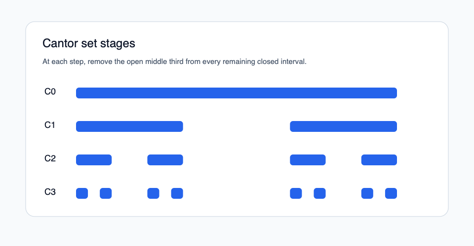
The first stages of the Cantor set construction

Figure. Each stage removes the middle third from every interval that survived the previous stage.

Read and try

Step through the Cantor set construction

The viewer shows how repeated middle-third removal creates a set that is small by length but large by cardinality.

Stage

C_0

Remaining intervals

Removed length so far

The limit set keeps exactly those points that can be written in ternary using only the digits 0 and 2.

Density in the real line

The next section introduces a different notion of largeness.

Definition

Dense subset of $R$

A subset $S\subset R$ is dense if for every $r\in R$ and every $\epsilon>0$ , there exists $s\in S$ such that

|r-s|<\epsilon.

This definition does not ask how many elements $S$ has. It asks whether elements of $S$ can approximate every real number arbitrarily well.

Equivalently, no matter where you stand on the real line and no matter how small a tolerance you choose, some element of $S$ lies within that tolerance.

Integers are not dense

Theorem

$Z$ is not dense in $R$

Take

r=\frac12,\qquad \epsilon=\frac14.

For every integer n,

\left|n-\frac12\right|\ge \frac12>\frac14.

So no integer lies within distance 1/4 of 1/2. Hence $Z$ is not dense in $R$ .

The proof only needs one failed target point and one failed tolerance. To show that a set is not dense, you do not have to check every real number. You only need to find a gap that the set cannot enter.

Rationals are dense

Theorem

$Q$ is dense in $R$

Let $r\in R$ and let $\epsilon>0$ . By the Archimedean property, choose $n\in N$ such that

n>\frac1\epsilon, \qquad\text{so}\qquad \frac1n<\epsilon.

Choose the largest integer $m_0$ satisfying

m_0\le nr.

Then

m_0\le nr<m_0+1.

Dividing by n gives

0\le r-\frac{m_0}{n}<\frac1n<\epsilon.

Thus

q=\frac{m_0}{n}\in Q

satisfies $|r-q|<\epsilon$ . Therefore $Q$ is dense in $R$ .

This proof shows exactly what density means: for any requested tolerance, a rational approximation can be chosen inside that tolerance.

Common mistake

Dense does not mean uncountable

The rationals are dense in $R$ , but earlier cardinality results show that $Q$ is countable. Density measures approximation, not cardinality.

The same idea can be restricted to a subset of the real line.

Definition

Dense in a subset

Let $T\subset R$ . A subset $S\subset T$ is dense in $T$ if for every $t\in T$ and every $\epsilon>0$ , there exists $s\in S$ such that

|t-s|<\epsilon.

Well-ordering

The last part of Chapter 6 turns from size and approximation to order.

Definition

Well-ordered set

Let $(X,\le)$ be a totally ordered set. We say $(X,\le)$ is well-ordered if every non-empty subset $S\subset X$ has a minimum.

This is stronger than merely being totally ordered. A total order lets you compare two elements. A well-order additionally says that every non-empty subcollection has a first element.

Worked example

Finite initial segments of $N$

In the von Neumann construction, a natural number n is identified with

n=\{0,1,\ldots,n-1\}.

Ordered by inclusion, this is the usual order on the finite initial segment. Every non-empty subset has a least element, so each finite n is well-ordered.

Theorem

The natural numbers are well-ordered

The usual order on $N$ is a well-order: every non-empty subset of $N$ has a minimum.

The proof is by contradiction using induction. If a non-empty subset $S\subset N$ had no minimum, induction would show that $0\notin S$ , then $1\notin S$ , then $2\notin S$ , and so on. Hence no natural number would lie in $S$ , contradicting non-emptiness.

Orders that are not well-orders

Theorem

$Z$ is not well-ordered by the usual order

The subset $Z\subset Z$ has no minimum. For any $n\in Z$ , the integer $n-1$ also lies in $Z$ and satisfies $n-1<n$ . Therefore no element can be first.

Theorem

$Q^+$ is not well-ordered by the usual order

The subset $Q^+$ has no minimum. For any positive rational q, the number q/2 is also positive rational and satisfies q/2<q.

The second example is especially important because all elements are positive. The failure is not caused by negative numbers. It is caused by an infinite descending process with no first positive rational.

Common mistake

A minimum is not the same as a lower bound

The set $Q^+$ has lower bounds in $R$ , such as 0, but $0\notin Q^+$ . A minimum of a set must belong to the set itself.

Countable sets can be well-ordered

Now separate two statements:

a particular order may fail to be a well-order;
the underlying set may still admit some other well-order.

Theorem

Every countable set can be well-ordered

If $X$ is finite, list it as

X=\{x_1,\ldots,x_n\}

and order the elements by their indices.

If $X$ is countably infinite, choose a bijection

f:N\to X.

Define

x\le_X y \quad\text{if and only if}\quad f^{-1}(x)\le f^{-1}(y) \quad\text{in }N.

This transports the well-ordering of $N$ to $X$ .

For example, $Z$ is not well-ordered by its usual order, but it is countable, so it can be well-ordered by choosing an enumeration of its elements.

The Well-Ordering Theorem

The chapter ends by connecting well-ordering to the Axiom of Choice.

Theorem

Well-Ordering Theorem

The Axiom of Choice is equivalent to the statement:

every set $X$ can be well-ordered.

One direction is direct. If every set can be well-ordered, then for a family of non-empty sets, well-order the union and choose from each member its least element. That gives a choice function.

The other direction uses the Axiom of Choice to choose an element from every non-empty subset of $X$ , then tries to build an order by repeatedly choosing the next unused element. This direction is more technical because making the construction precise requires transfinite recursion, which is beyond the course.

Common mistake

The Well-Ordering Theorem is not saying the usual order works

The usual order on $R$ , $Z$ , or $Q^+$ may fail to be a well-order. The theorem says that some well-order exists, assuming the Axiom of Choice. It does not give a familiar or computationally useful order.

Quick checks

Quick check

At stage n of the Cantor construction, how many intervals remain and what is the length of each one?

State both quantities in terms of n.

Solution

Answer

Quick check

Why does the proof that $Z$ is not dense only need to examine `r=1/2` and `epsilon=1/4`?

Use the definition of not dense.

Solution

Answer

Quick check

Why is $Q$ dense in $R$ even though $Q$ is countable?

Name the two different ideas being compared.

Solution

Answer

Quick check

Why is the usual order on $Z$ not a well-order?

Identify a non-empty subset with no minimum.

Solution

Answer

Exercises

Quick check

Use the ternary description to decide whether $(0.202020...)_3$ lies in the Cantor set.

Explain which digits matter.

Solution

Guided solution

Quick check

Prove that $Q^+$ is not well-ordered by its usual order.

Use the same ternary-expansion idea.

Solution

Guided solution

Quick check

Let $X$ be countably infinite and let $f:N\to X$ be a bijection. Why does the transported order on $X$ become a well-order?

Use the well-ordering of $N$ .

Solution

Guided solution

Read this after 2.2 Functions and relations, 4.2 Upper bounds, supremum, and infimum, and 4.3 Completeness and gaps in Q. Then continue to 7.1-7.2 Binary operations, monoids, and groups.

6.4-6.7 Intervals, Cantor set, density, and well-ordering

MATH1090: Set theory

Closed intervals and half-closed intervals

Closed interval

Do not treat interval notation as decoration

Intervals and cardinality

The interval (0,1) has cardinality |R|

Why boundedness does not control cardinality

The Cantor set construction

Cantor set

Endpoints survive

Ternary expansions and membership in CCC

Ternary description of the Cantor set

The length paradox

The Cantor set has cardinality |R|

The Cantor set has the same cardinality as RRR

Zero length does not mean countable

View the stages

Step through the Cantor set construction

Density in the real line

Dense subset of RRR

Integers are not dense

ZZZ is not dense in RRR

Rationals are dense

QQQ is dense in RRR

Dense does not mean uncountable

Dense in a subset

Well-ordering

Well-ordered set

Finite initial segments of NNN

The natural numbers are well-ordered

Orders that are not well-orders

ZZZ is not well-ordered by the usual order

Q+Q^+Q+ is not well-ordered by the usual order

A minimum is not the same as a lower bound

Countable sets can be well-ordered

Every countable set can be well-ordered

The Well-Ordering Theorem

Well-Ordering Theorem

The Well-Ordering Theorem is not saying the usual order works

Quick checks

At stage n of the Cantor construction, how many intervals remain and what is the length of each one?

Answer

Why does the proof that ZZZ is not dense only need to examine r=1/2 and epsilon=1/4?

Answer

Why is QQQ dense in RRR even though QQQ is countable?

Answer

Why is the usual order on ZZZ not a well-order?

Answer

Exercises

Use the ternary description to decide whether (0.202020...)3(0.202020...)_3(0.202020...)3​ lies in the Cantor set.

Guided solution

Prove that Q+Q^+Q+ is not well-ordered by its usual order.

Guided solution

Let XXX be countably infinite and let f:N→Xf:N\to Xf:N→X be a bijection. Why does the transported order on XXX become a well-order?

Guided solution

Related notes

Prerequisites

Key terms in this unit

More notes in this series

The interval `(0,1)` has cardinality `|R|`

Ternary expansions and membership in $C$

The Cantor set has cardinality `|R|`

The Cantor set has the same cardinality as $R$

Dense subset of $R$

$Z$ is not dense in $R$

$Q$ is dense in $R$

Finite initial segments of $N$

$Z$ is not well-ordered by the usual order

$Q^+$ is not well-ordered by the usual order

Why does the proof that $Z$ is not dense only need to examine `r=1/2` and `epsilon=1/4`?

Why is $Q$ dense in $R$ even though $Q$ is countable?

Why is the usual order on $Z$ not a well-order?

Use the ternary description to decide whether $(0.202020...)_3$ lies in the Cantor set.

Prove that $Q^+$ is not well-ordered by its usual order.

Let $X$ be countably infinite and let $f:N\to X$ be a bijection. Why does the transported order on $X$ become a well-order?